QUALITY CHECKING METHODS USEFUL FOR ALL PROJECTS

Hello All...

         Here we shall discuss effective Quality Checking Methods in Detail. Master these methods as they were useful for a lot of data entry projects. Don't ever pay attention to the headers.

        Let me start with first lesson to day.. These methods were useful to small BPO Centers, Quality Checking Staff and Home Based Data Entry Operators as well as those who wants to become experts in MS Excel up to some extent. These methods were accurate and works well with MS Office 2007. So, please be sure that you are using Office 2007..

         What ever the project name and kind of work may be, all the data fields can be defined in  2 kinds of fields......Unique and Random.....

          Unique Values Fields: These fields will have fixed set of values and only these few values would repeat. Remember that these fixed set of values would have a specific format and there will be no variation through out the entire process. Gender Fields (Male, Female), CreditCardType Fields (MasterCard Gold Card, MasterCard - Platinul Plus, MasterCard Titanium, Visa Gold Credit card) Residence Type (Apartment, Condominium Single Family Home, Double Family Home) etc..etc.. can be defined as Unique Values Fields.

           Random Values Fields: The word Random is used here is to denote that the values in this kind of fields would not repeat. For example, names of the persons, email address, residential addresses, etc..etc...

        Now, lets us discuss about the various common fields found in every form filling process.

        1. Transaction/Reference Number: For each and every transaction, there should be some kind of reference. It may some times has a field name as Form Number, File Number, Invoice Number, Bill Number, Reference Number., etc..etc.. But, what ever the name may be, almost all the processes would have a numeric (means those fields which contains only numbers) and alpha numeric fields (means those which have both numbers and alphabets). As I had said earlier, in most processes, they would take extra care while providing the data to include 1s (number One), 0s (zeros), lower case l (as in the word lady), upper case I (as in the word India), upper case O (as in the word Owl), and lower case o (as in the word rod) apart from hyphens (-) and underscores (_) as these few alphabets, numbers and special characters would look similar in most fonts, especially in those fonts used in these projects.  In a lot of processes there will also 2 initial fields namely Image/File Number and Form/Record Number. These two fields denotes the source data reference of a particular form or record. Each form/record's data should be represented precisely with these two fields - that means, even if the entire form doesn't have a mistake, if the two fields have an error, the entire form would be treated as an error. So, be extra cautious with these two fields.

           2. Names Fields: Usually, for each and every transaction, there should be an end consumer/client. So, if it is a customer name in some process, and in some other processes it may have a different name -  agent name, doctor name, patient name, relative name, neighbor name, friend name, father or mother name. Only the header - by which a field represents would change.  Here, the problem isn't the name it self. we should not bother about the field name either. In this field, there will be further confusing instructions. In some process, the vendor asks us to enter the data as it was in the source file without any formatting. In some other cases, they would instruct us to use Proper Case - means, every first letter in each word should be capitalized and remaining letters should be in lower case; or Upper Case - means each and every letter should be in Capital Letters only; or even Lower Case - means each and every letter should be entered in lower case only. You should be carefully enough to differentiate between Upper Case and Lower Case as a few alphabets such as J (Joy),  I (India), Z (Zeal), X (Xerox), C (Cat), V (Van) would look similar in both cases.

          3. Initials: This field is a sub field of names field. In this field, you should enter each first letter of the all words in the name field with a dot in between in Upper Case only. Here also, there will be some confusing instructions would be given to operators. In some cases, some vendors instructs us to omit ordinals - means I, II, III, IV as in King George I or James II; Suffixes and Prefixes - Dr., Mr., Mrs., Ms., Jr., Sr., Br., Mc., etc..etc..,

          4. Dates Fields: On an average, a lot of processes would have 2 different dates fields. Usually they instruct us to enter a date field in MM/DD/YYYY and the other in DD/MM/YYYY format. That means, we shall enter a date in the first instance in Month followed by Date followed by Year - in american style and in the other instance we shall enter the Date followed by Month followed by Year in Indian style. Here, you should be careful enough to use only either slash (/) or hyphen (-) as per the vendor's instruction. Using both or other than prescribed would be treated as error. Here is an interesting point to remember. Those fields that has to be entered in MM/DD/YYYY format will be provided in DD/MM/YYYY format in the source file only to confuse us. That too, all the dates values in this format will be with in 12 - that means there will be no date value bigger than 12. In the DD/MM/YYYY format also the source data would be in reverse, but, dates values will be upto 31.

           5. Email Field: This usually follows a name field. In this field one should be careful enough with the vendors instructions, as they usually try to confuse us by their instructions - some times they asks us to omit spaces and correct a few values, and at other instances they instruct us not to do any corrections.

            6. Address: Almost all the processes would provide United States of America addresses. You should be aware of typical addresses of USA. -  as they would end up with Ct (Court), Ln (Lane), Blvd, St (Street), Sq (Square), Ave (Avenue). So, these ending street names should not be entered in the City Field which usually follows the Address Field.

             7. City: This field always follows the Address field. These were all USA Cities. You will be familiar with these cities names in a few days, once you get down to working on the projects.

             8. State: This filed also always follows the State Field. These states were all USA states and will be in abbreviated form. So, there should not be more than 2 characters in this field.

             9. Country: This field would present in only a few processes, followed by State field always. In most projects, the country name will be USA by default.

             10. Zip Code: These were all USA Zip Codes. Usually a zip code will have 5 numerals, but, in some cases there will be more or less than 5 characters, only to make things pretty difficult for the operators. In some projects there will be 2 zip codes fields namely Zip 1 and Zip 2.

                12. Phone Number: This field will have 10 numerical values in this format (123) 456-7890. The data should be entered exactly in this format only although in some instances the supplied data would not be in this format.

                 13. SSN (Social Security Number) and Credit Card Number: There two fields would look similar. Both are numerical values. Usually a SSN Value would have 11 numerical where as Credit Card Number will have 16 numerical. There willl be some values with more or less numerical also.

                 14. Banks Name: This field usually denotes the credit card issuing authority namely MasterCard Titanium, Visa Gold Credit card, MasterCard Gold Card, MasterCard - Platinul Plus and rarely at one or two forms another value Credit Card Type will come in this field.

                 15. Amounts: There will be a lot of fields in this category, but one should remember that these were all only numerical fields.


                  16. Gender Fields: Here only 2 values - either Male or Female would be present. In general projects with some kind of medical data will have this field.

                  17. Age Fields:  This will be numerical values field with ages of a person. This field also happens to be in medical projects.

                   18. Credi Rating : Usually there will be four unique values for this field, namely  Excellent, Fair, Good, Poor.

                  19. Remarks: This field used to mention only if we find irrelevant data in any field or missing data in a field. Other wise, we shall enter only N.A.



           Now, open the attachment " Doc 1 - Medical Sales Pro" and we shall discuss the fields so that you would get an idea about the fields.

                                  Here is the download link:
DOC 1 - MEDICAL SALES PRO

                                  Here is the download link to Images for this File:
http://www.mediafire.com/?4z92gadi1gn1abw


         Before to start working on this file, we shall apply some formatting here. Select the whole sheet (Press and hold Ctrl Key and press A twice), change the font face to Verdana and Font Size to 14. Then press the vertical columns separator between any 2 columns twice to adjust all the columns automatically according to their corresponding data width. Now, select the first two columns and align them to right side (press Alt, H,AR). Now move the cursor to Cell C2 and then open Freeze Panes option (press Alt, W, F, F) to freeze the header line and first 2 columns. Now, let us start the QC Process... Here, the first 2 fields are File Number and File Sub Number (Columns A and B) as discussed above in the first point. The first field File number means, it represents the source image number, and the second field File Sub Number (Record Number) denotes the Form number in that particular image. Remember to enter the forms in the exact order/serial as they were in the source images. Suppose, if you miss to enter a form in the middle, you should not enter it in the end as it changes the order of the entire image and the following forms in that image would be treated as errors in the QC Process. (No of forms multiplied by the total number fields) If such a thing happens, you should delete the remaining forms first and enter the missing form in its position then re enter the following forms.

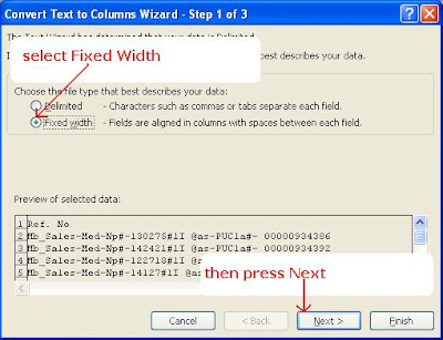Then the next field is Reference Number - this field also discussed above in the 1st point. Examine carefully a few reference numbers for a while, and you would notice that there are a lot of lower case l (lady) upper case I (India) and 1s (one) zeros (o) as discussed above apart from hyphens and underscores. It looks very lengthy too. No problem, what ever the length of such fields may be. Because, if we carefully observe them only 2 variations were occurring there. From the beginning to middle is repeating(Mb_Sales-Med-Np#-l) as shown in the figure above marked with red lines, then the numerical values changes (marked with Blue Lines) and then from there to end (#1I @as-PUC1a#- 00000) (again marked with red lines) is same, only the last numerical values are changing.  For this kind of fields, there is a specific technique to cross check pretty easily. Now go to the excel, press Shift+F11 to insert a new sheet to do qc work, copy columns a,b and c (File number, Record Number, Reference number fields - press Ctrl+Home to move cursor into Cell A1, then press Ctrl+Space to select column A and then  by press and hold down the shift key press Right Arrow Key 2 times to select Columns B and C. Now, press Ctrl+C to copy, press Ctrl+Page Up to open newly inserted sheet, press Ctr+V to paste the copied data. Now, again copy the Column C data here and paste the same into Column D. Now open the Text to Columns Option in Excel - press Alt, A, E consecutively. (Please remember carefully that when ever I ask you to press a combination of keys with a plus symbol in between them, that means you have to press and hold the first control key while pressing the followed key and when ever I use a comma that means you should not press and hold the previous key. Got it? To make things easier to understand, in the first instance I had asked you to press Ctrl or Shift followed by plus symbol (=) that means you have to press and hold the Ctrl or Shift Keys while pressing the followed keys F11 or Page Down or C or V. But, in the second instance I said this combination keys in a different way using comma symbol (,) which means you should not press and hold Alt key while pressing A and E. Just press Alt key once, release it then press A and E simultaneously to perform the entire sequence of commands) Now, you would notice a dialogue box pops out with a name "Convert Text to Columns Wizard - Step 1 of 3" as show in the figure below..  This tool is very useful in a lot of ways. I will explain as and when the situation arises. Now, we use this tool to bifurcate a column into several columns as per out wish. Look at the dialogue box carefully, you would notice 2 options at the top, namely Delimited and Fixed width. These are 2 types used to in bifurcation process. If we select Delimited, we shall have to mention a fixed delimiters such as Tabs, Space, Comma, dot or any other special characters. This option particularly useful when the data is in variable length. Look at the excel carefully (Drag this dialogue box to the right side of the screen) and you would  notice that there is no variation in length till Np#-l. But, after that the numerical values were of varied length from 2 to 5 digits. So, now, select the Fixed width option as shown in the figure, and press next.
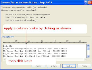Now, use the mouse and move the cursor and point it between l and numerical and press (left key) once. You would notice a line appears here. Even if you fail to click exactly at the above said position, no problem, you can move it in sideways by pointing the cursor over the line and dragging it by holding the left key (in the mouse). Now press next.  Here you will again get 4 options to choose from as shown in the figure aside. 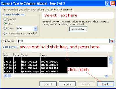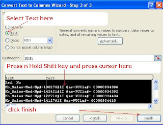Select text always. We use the other 3 options as and when required and I will explain them later. The first part usually be selected with general tag to it. Now, press and hold the Shift key and then move the cursor over the second part and click on it to select. Now, you would see both parts were selected. Now, select Text in the top 4 options and click finish. Column D now bifurcated into 2 columns. Select the whole sheet and change the font face and size. (Press Ctrl+A 2 times to select the entire sheet). Apply Filter Command - Alt, A, T, go to Cell D1 and press Alt+DownArrow. You would get a drop down menu with the unique values of the column. This sheet has 4040 forms and if in case, in any form, this first part has variations (other than "Mb_Sales-Med-Np#-l") you would see them all. If in case, all the forms has been entered correctly, you would see only one value in the drop down menu. You can also cross check this option to make sure you are familiar enough as we have to do a lot of things with this option, go to a cell in column D and edit it according to your wish. Now, press Ctrl+UpArrow to move the cursor to Cell D1 and again press Alt+DownArrow to open drop down menu of Filter Command Options. You would now notice different values. OK? When ever we use this option to cross check the uniqueness of values, we shall remove the tick box against the only one correct value, and press enter. By doing this, all those correct entries will be omitted and only those with errors would be displayed. We can edit these few error fields pretty easily. After editing these error fields go to Cell D1 again and press Alt+DownArrow to cross check the uniqueness. There should be only one value. If there are still more values other than the unique value, you are only half done the editing. K?

         Now, lets move to second part. Here You would notice that the data here is not in fixed length. Also, to make things easier, if we extract the numerical values which are variable in nature would be better to cross check the data effectively. For this, to extract first numerical value field, replace the hash symbol before 1I with a space - go to cell E1, press Ctrl+Space to select the entire column, press Ctrl+H to toggle Find and Replace

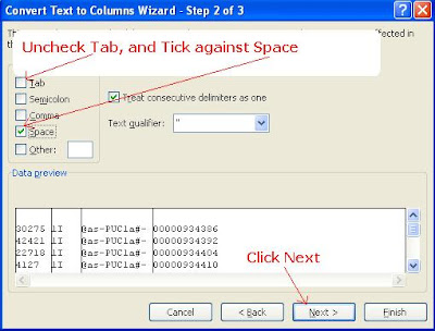Option (see Figure beside), enter #1I in find what box and apply a space and 1I in Replace with box, press Alt+A to replace all. Now, all the hash symbols before 1I would be replaced by a space. Now, open the Text To Columns Tool (Alt, A, E) and select Delimited press next. Un check the tick against Tab option, and put a tick against Space option and press next. Now press and
hold shift key and hover the cursor in the last column and press left key in the mouse to select all the four columns and select text. Here you may wonder, why should we select text option, as the data was in general format. When ever we select text option, the zeros before a numerical value would not be formatted/omitted. If we do not select text, all the zeros before a numerical will be deleted and it will be hard to cross check the data precisely. Now, press finish. So, again 4 new columns were created. Re aply the filter to include these four new columns. Always remember to apply filter command to the entire data columns, other wise, if we sort the data, the rows will be mismatched. To over come this problem, when ever a new column is created/inserted in the end, we have to re apply the filter command to cover the new columns. Now, go to Cell F1 and check for the unique values. There should be only one Value that is 1I. If you see any other values then edit the in the same manner as suggested in the previous instance of column D. Repeat these steps with column G. and after completion, delete the columns D, F and G as there is no further usage with them and if left, they will confuse us. So, with these steps, we had extracted the two numerical values only. In a lot of projects, when we sort these numerical values in ascending or descending order, another field (names fields, email, address...what ever it may be) will show you a specific order. That means, that field values should be in correct position. To make things easier, for instance, assume that there are 1 to 9 in column A and a to i in column B. If we sort the column a in ascending order, then column b also should show its values in ascending order unless there were any errors at the time of entry. This is a very useful short cut to locate exactly where a mistake has occurred indeed. Let us see how this method works actually. Delete the columns D, F, G from the new sheet (Sheet 1). Copy the Columns E and H (the 2 numerical values fields) and paste them before or after the Reference Number Field in the first sheet (Sheet 596) Reapply the filter command and sort the first numerical value. Now move the cursor to Column J (Dispatch By Field) and you could notice that all the names values in that column was also sorted in ascending order. That means, if we did a mistake either in the first numerical values or here in the Dispatch By field, this principle would be false. Other wise it works well. In other words, follow this. Insert another sheet (press Shift+F11). This will be Sheet 2. Now, sort the first numerical values and then copy the first 2 columns (File Number and Record Number) from Sheet 596. Paste them in Columns A and B in Sheet 2. Now, go back to Sheet 596, sort the Column J in ascending order (Dispatch by Field). Now, copy the First 2 columns A and B (File Number and Record Number) and paste them Columns C and D in Sheet 2. Let me know how you are following these steps now. Please download the following attachment, and check it with your work. It will have Sheet 1 and Sheet 2, with the columns discussed above. If your excel sheet doesn't match with this attachment, please go back and re try it till you get the result. Here is the link to download the attachment:
DOC 1 - WITH SHEET 1 & 2

        Now, go to Cell E1 of Sheet 2, press Alt, M, N, N to enter a new formula. Using the formulas in MS Excel makes things pretty easier. You can enter a formula directly into Cell E1 and copy it till the end. But, if we sort the columns, these formulas cells of references would change and the results of the formula would be false. To over come this trouble, always use the formulas manager. Now, let us go back to the formula manager. Enter a name of your choice in Name Field. Be sure to enter a name with less characters as it will be easy to enter and make sure the abbreviated names should correspond to the task we are going to do. Here, the task is to  match whether Cell A1 and C1 are same or not. So, use Ex - exact or Eq - Equal as the formula name. Here I am assume that you are using Ex as the formula name. Then leave Source and Comment fields and go go Refers To box and enter =a1-c1 and press enter, then escape to return to the working sheet. Now, in Cell E1 enter this new formula (=ex). Copy this formula and paste it into Cell F1. Now, copy both E1 and F1 Cells, press left arrow key once (to move the cursor into Cell D1), press Ctrl+Page Down to reach the end of the document, go to E column. Now, press and hold Shift key and then press Right Arrow key once to select both E and F cells. Now, holding the shift key, press and hold Ctrl and then press UpArrow. (Shift+Ctrl+UpArrow, all at once) and paste (Ctrl+V). Now, we had applied the formula in both Columns E and F. If both Numerical Values and Dispatch By fields were entered correctly, this formula would show TRUE. If there is a mistake, then it will shows FALSE. Although, there were a very few exceptions to this formula's accuracy, it works well at most times.

          Now, lets do some editing practically.. Leave aside your excel sheet (in case, if you fail to execute the above methods precisely) and open the second attachment.

          Here, you will find 3 sheets, namely Sheet 2, Sheet 1 and 596. Now, go to Sheet 2 and apply the formula  in both columns E and F. Now open Find and Replace Dialogue Box (Press Ctrl+H) and enter FALSE in find what dialogue box. Open options (Alt+T) and then go to look in (Alt+L), select Values (you can press V to select), and hit enter.  Now, you would move directly to the first instance of an error at File Number 173 and Form Number 5 at Row No. 60. Now, hit escape key to close the find n replace dialogue box.  Go back to sheet 596 (press Ctrl+PageDown 2 times) and go to any cell in Column A (File Number), select the entire column (Ctrl+Space), open FindWhat option (Ctrl+F) enter 173 in Find What box. Now, you may have a doubt about the previous steps of selecting column A before searching for a value. If we do not select specific area where to search the value, all the values at other fields that matches our search term will be displayed. To over come this problem, in most cases, we would select the specific columns to search before opening the FindWhat Dialogue Box. When you hit enter key, you will go to first form of File number 173 at Row Number 3863. Press down arrow till you  each the form number 5 at Row Number 3867. Now, press Right Arrow key to move the cursor in to DispatchBy Field., you can see that alfredr mejia jr in the Dispatch by field. open the image 173 (download the images of this project with the link provided above). According to the data provided, it should be alfred r mejia jr although there seems to be no space between alfred and r. Edit the dispatch by field and come back to Sheet 2 again to continue the cross checking process. Move the cursor into Cell C60, Press Shift+RightArrow once to select D60, Press Ctrl+Shift+DownArrow to select the all the values beneath the Row No 60, Cut them (Ctrl+X), press down arrow once to move the cursor in to Cell C61 and paste (Ctrl+V). By doing this we are trying to match both values at Columns A & C and B & D. Repeat the same steps to move down values of Column A and B at Row No. 64. (Cut them From and paste them at Row No. 65. To match both values, this is one kind of method to follow. There is another method also. You can delete the values of Columns C & D at Row No. 64 by cut n pasting the values of Row No. 65 to till the end into Row No. 64. Either is way correct, but, one has to follow either of this method according to the situation. I will explain them in detail later. Now, you could notice that, when you re arrange the values of Columns C and D, the formulas at Columns E and F shows you TRUE automatically. If in case we do not used the formula manager while applying the formulas, such a thing never happens. Got it? You can check it by entering the formula manually [(=a1=c1) directly into Cell E1 and (=b1=d1) directly into Cell F1. Copy the two cells and paste the same till Row No. 4041]  to make things easier for understanding and to have a better idea to deal with the formulas. Now, lets get back to the cross checking.

     In most projects, the first field always happens to be a numerical or alpha numerical value. If it is a alpha-numerical field (contains both alphabets and numbers, usually alphabets followed by numbers), always bifurcate it into two columns - alphabets and numbers so that it will be easier to cross check the data. Always try to find out if there is any order, pattern or sequence in the numbers. In this sample field you would notice that these numbers were all in multiples of 6. If in case, an error occurs, we can find it pretty easily by finding out the difference of 2 consecutive cells as described below. Now, go back to Sheet1 and go to Cell F2, open the Name Manager (Alt, M, N, N) in the Name (formula) field give a catchy name, as we are deducting (minus) the cell values, MN would be apt here. Skip Scope and Comment Fields and go directly to Refers to Field (Press Tab 3 times after entering MN) and enter this formula = E3-E2 and press Enter and press Escape to close the Name Manager. Now, in Cell F2 enter =MN, copy it and paste it till Cell F4041 (after entering the formula =MN press enter, Ctrl+C, LeftArrow, Ctrl+DownArrow, RightArrow, Ctrl+Shift+UpArrow, Ctrl+V). Now, reapply the filter command to include F Column. Go to Cell F1, and press Alt+DownArrow, DownArrow...Now, you could see the numbers in multiples of 6 ie..6 12 18 24 36...so on.. Here, if you find any value other than the multiples of 6, there was an error. So, go directly to that cell, and edit it. You need to check those higher values of 24, 36 etc...as  it may happens to be, at times, if an operator misses a form. So, we shall cross check those values with the images.

      In general, this reference number always happens to be either in ascending or descending order. We shall also check whether this principle applies correctly or not by this method. Now, move the cursor in to cell G2. Open the name manager. Always remember to reorder the Excel sheet sorted in ascending order...sort form number first and then file number. If you fail to do so when ever you apply the filter command and sort a single or multiple columns, you would not get proper results with the next steps. So, always be sure to keep first two columns sorted in ascending order. Ok.. Now, open the Formula Name Manager (Alt, M, N, N) enter a formula name...as we are now trying to check whether the corresponding cell is higher than the previous cell or not, it would be apt to give LS (less than) as the formula name.. Enter the formula = E2 less than E3 (use the less than symbol instead of typing less than) and repeat the steps described above.

          That is it for now as far as the Reference Field is concern. Practice them for quite a few hours till you are familiar with applying the formulas, key board short cuts to navigate quickly between rows and columns. In the following steps, these keyboard short cuts would not be mentioned as its just waste of time to repeat them every time.